example003_noisy_backward

This example shows how to filter and transform noisy data. It illustrates how noisy input data can lead to large errors of the backward transform result, and how filters can be used to -- at least visually -- alleviate those errors.

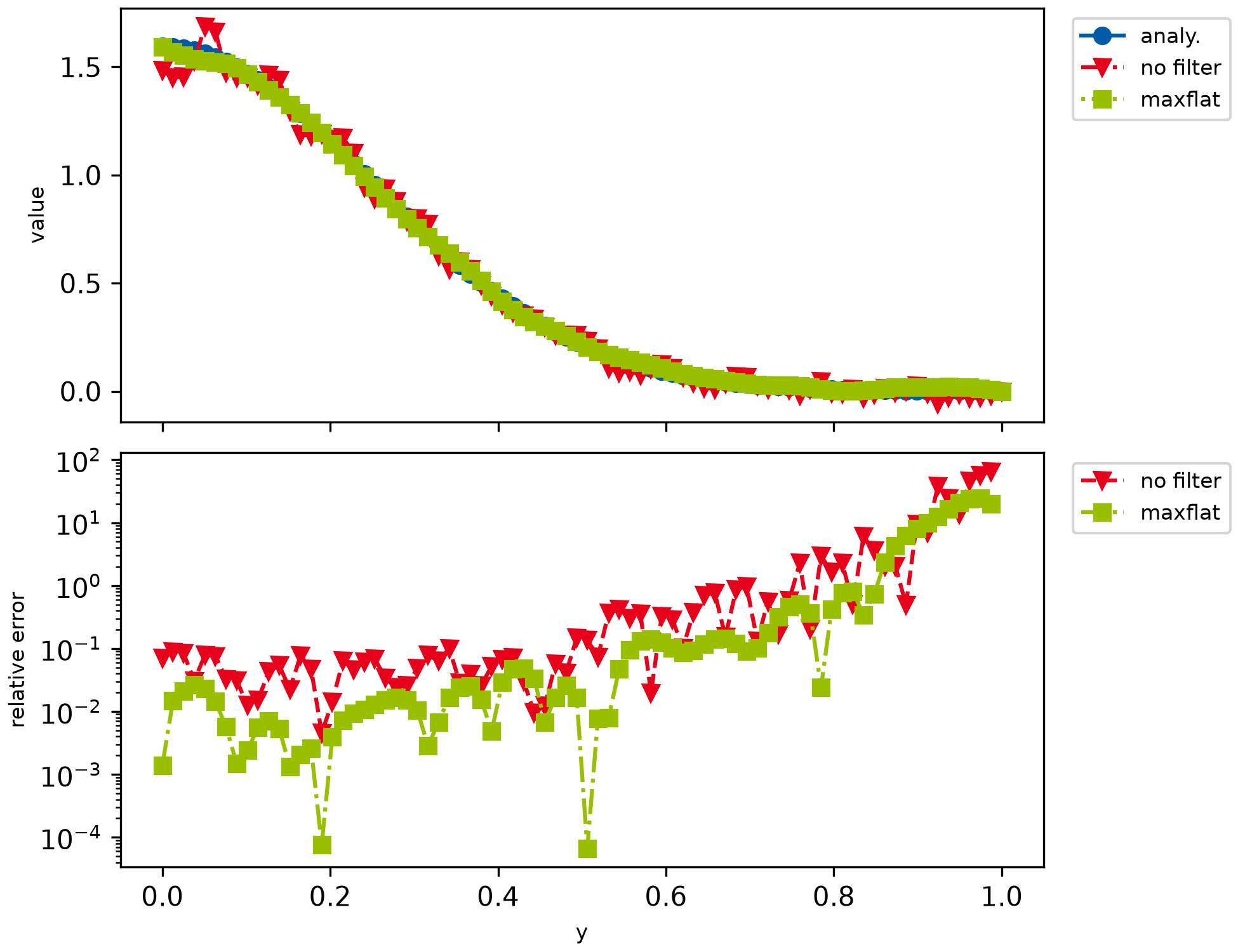
Maximally flat filters have been calculated as described in a paper by Hosseini, and a small Mathematica script of the calculation is provided in the additional materials.

############################################################################################################################################
# Example which calculates backward Abel transform of noisy data.
# This is a typical use case for many experimental line-of-sight measurements.
# openAbel doesn't inherently provide any filtering or smoothing, but one
# can achieve good results with manual noise-robust numerical derivatives.
############################################################################################################################################


import matplotlib.pyplot as mpl
import numpy as np
from scipy.special import erf

import openabel

############################################################################################################################################
# Plotting setup
# This block can be ignored, it's just for nicer plots.

params = {
    "axes.labelsize": 8,
    "font.size": 8,
    "legend.fontsize": 8,
    "xtick.labelsize": 10,
    "ytick.labelsize": 10,
    "text.usetex": False,
    "figure.figsize": [6.5, 5.0],
}
mpl.rcParams.update(params)
# Color scheme
colors = [
    "#005AA9",
    "#E6001A",
    "#99C000",
    "#721085",
    "#EC6500",
    "#009D81",
    "#A60084",
    "#0083CC",
    "#F5A300",
    "#C9D400",
    "#FDCA00",
]
# Plot markers
markers = ["o", "v", "s", "D", "p", "*", "h", "+", "^", "x"]
# Line styles
linestyles = ["-", "--", "-.", ":", "-", "--", "-.", ":", "-", "--", "-.", ":"]
lw = 2

############################################################################################################################################

# Parameters
n_data = 80
x_max = 1.0
shift = 0.0
sig = 1.0 / 4.0
step_size = x_max / (n_data - 1)
forward_backward = 2
noise_amp = 0.01

abel_obj = openabel.Abel(
    n_data,
    forward_backward,
    shift,
    step_size,
)  # Backward Abel transform where user inputs derivative


# No filtering
der = np.asarray([0.5, 0.0, -0.5]) / step_size
xx = np.linspace(
    -step_size * (der.shape[0] - 1) / 2,
    x_max + step_size * (der.shape[0] - 1) / 2,
    n_data + (der.shape[0] - 1),
)
data_in = np.exp(-0.5 * xx**2 / sig**2)
np.random.seed(2202)
data_in_with_noise = data_in + noise_amp * np.random.randn(n_data + (der.shape[0] - 1))

# Take derivatives
data_in_d = np.convolve(data_in_with_noise, der, mode="valid")

# Backward transform
data_out_no_filter = abel_obj.execute(data_in_d)


# Maximally flat filtering
# The length of this filter should be adjusted to the noise.
# For more information see documentation and orignal maxflat paper https://ieeexplore.ieee.org/document/7944698/.
der = (
    np.asarray(
        [
            4.76837e-7,
            9.53674e-6,
            0.0000901222,
            0.000534058,
            0.00221968,
            0.00684929,
            0.0161719,
            0.0295715,
            0.041585,
            0.0431252,
            0.0280313,
            0.0,
            -0.0280313,
            -0.0431252,
            -0.041585,
            -0.0295715,
            -0.0161719,
            -0.00684929,
            -0.00221968,
            -0.000534058,
            -0.0000901222,
            -9.53674e-6,
            -4.76837e-7,
        ],
    )
    / step_size
)
xx = np.linspace(
    -step_size * (der.shape[0] - 1) / 2,
    x_max + step_size * (der.shape[0] - 1) / 2,
    n_data + (der.shape[0] - 1),
)
data_in = np.exp(-0.5 * xx**2 / sig**2)
np.random.seed(2202)
data_in_with_noise = data_in + noise_amp * np.random.randn(n_data + (der.shape[0] - 1))

# Take derivatives
data_in_d = np.convolve(data_in_with_noise, der, mode="valid")

# Backward transform
data_out_max_flat = abel_obj.execute(data_in_d)

# Analytical result
xx = np.linspace(step_size * shift, x_max, n_data)
data_in = np.exp(-0.5 * xx**2 / sig**2)
data_out_ana = data_in / np.sqrt(2 * np.pi) / sig * erf(np.sqrt((x_max**2 - xx**2) / 2) / sig)


# Plotting
fig, axarr = mpl.subplots(2, 1, sharex=True, layout="constrained")

axarr[0].plot(xx, data_out_ana, color=colors[0], marker=markers[0], linestyle=linestyles[0], label="analy.")
axarr[0].plot(xx, data_out_no_filter, color=colors[1], marker=markers[1], linestyle=linestyles[2], label="no filter")
axarr[0].plot(xx, data_out_max_flat, color=colors[2], marker=markers[2], linestyle=linestyles[3], label="maxflat")
axarr[0].set_ylabel("value")
axarr[0].legend(loc="upper left", bbox_to_anchor=(1.02, 1.0))

axarr[1].semilogy(
    xx[:-1],
    np.abs((data_out_no_filter[:-1] - data_out_ana[:-1]) / data_out_ana[:-1]),
    color=colors[1],
    marker=markers[1],
    linestyle=linestyles[1],
    label="no filter",
)
axarr[1].semilogy(
    xx[:-1],
    np.abs((data_out_max_flat[:-1] - data_out_ana[:-1]) / data_out_ana[:-1]),
    color=colors[2],
    marker=markers[2],
    linestyle=linestyles[2],
    label="maxflat",
)
axarr[1].set_ylabel("relative error")
axarr[1].set_xlabel("y")
axarr[1].legend(loc="upper left", bbox_to_anchor=(1.02, 1.0))

mpl.savefig("example003_noisy_backward.png", dpi=300)

mpl.show()