example006_simple_forward_and_backward

This example applies the forward transform to a Gaussian and then the backward transform to the result, and compares the round trip with the input. The backward transform differentiates its input numerically, which amplifies the small error of the forward transform; the round trip is still accurate to about 1e-8 over most of the domain. Towards the end of the domain, where the Gaussian is vanishingly small, the truncation of the integration domain shows in the relative error.

############################################################################################################################################
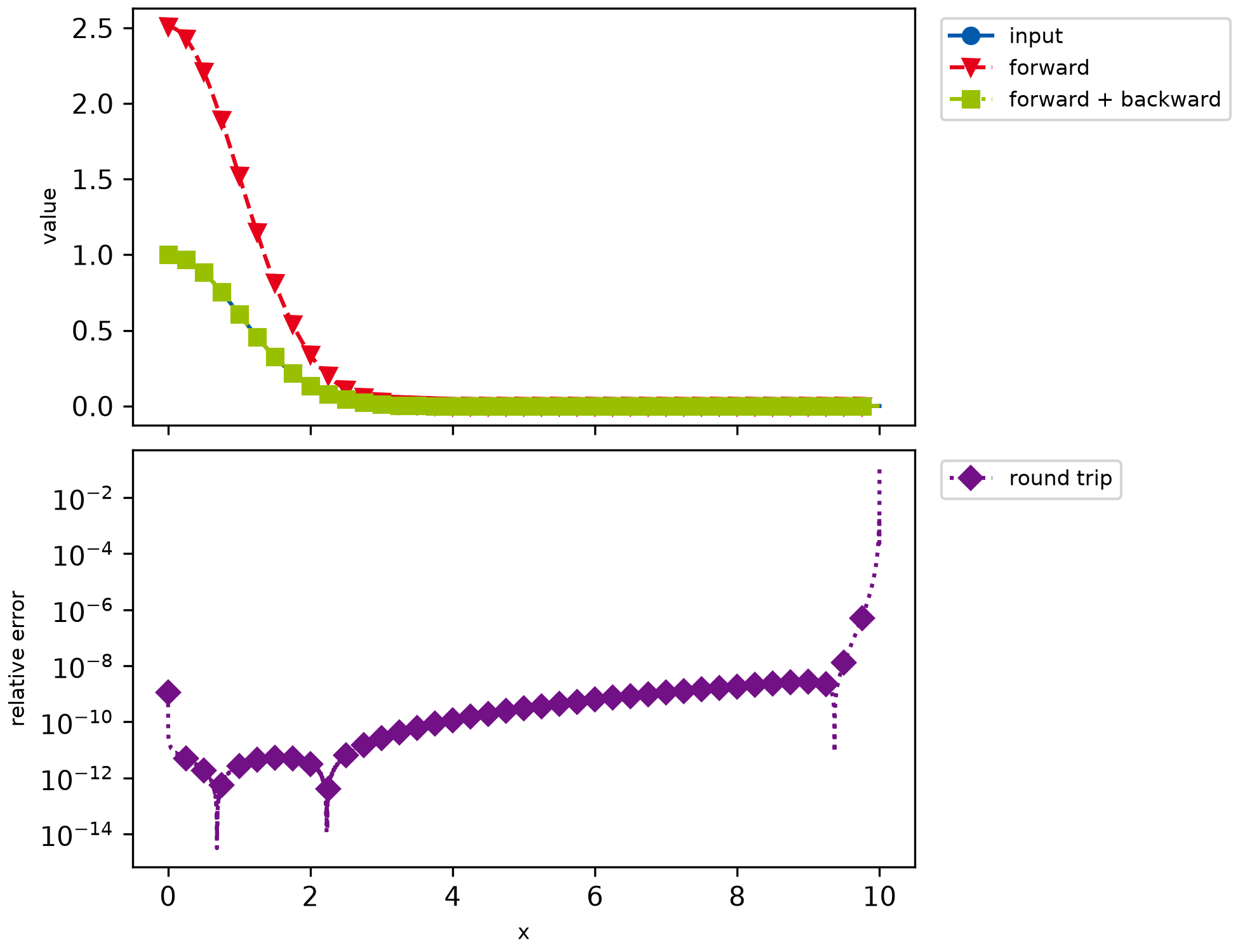
# Simple example which applies the forward and then the backward Abel transform to a Gaussian.
# The round trip is compared with the input. Mostly default parameters are used.
############################################################################################################################################


import matplotlib.pyplot as mpl
import numpy as np

import openabel

############################################################################################################################################
# Plotting setup
# This block can be ignored, it's just for nicer plots.

params = {
    "axes.labelsize": 8,
    "font.size": 8,
    "legend.fontsize": 8,
    "xtick.labelsize": 10,
    "ytick.labelsize": 10,
    "text.usetex": False,
    "figure.figsize": [6.5, 5.0],
}
mpl.rcParams.update(params)
# Color scheme
colors = [
    "#005AA9",
    "#E6001A",
    "#99C000",
    "#721085",
    "#EC6500",
    "#009D81",
    "#A60084",
    "#0083CC",
    "#F5A300",
    "#C9D400",
    "#FDCA00",
]
# Plot markers
markers = ["o", "v", "s", "D", "p", "*", "h", "+", "^", "x"]
# Line styles
linestyles = ["-", "--", "-.", ":", "-", "--", "-.", ":", "-", "--", "-.", ":"]
lw = 2

############################################################################################################################################

# Parameters
n_data = 10000
shift = 0.0
x_max = 10.0
sig = 1.0
step_size = x_max / (n_data - 1)

# Create the Abel transform objects, which do all precomputation possible without knowing the exact data.
# '-1' is the forward transform, '1' the backward transform (similar definition as in FFT libraries).
abel_obj_fw = openabel.Abel(n_data, -1, shift, step_size, order=3)
abel_obj_bw = openabel.Abel(n_data, 1, shift, step_size, order=3)

# Input data
xx = np.linspace(shift * step_size, x_max, n_data)
data_in = np.exp(-0.5 * xx**2 / sig**2)

# Forward transform, then backward transform of the result (which differentiates its input numerically).
data_fw = abel_obj_fw.execute(data_in)
data_bw = abel_obj_bw.execute(data_fw)


# Plotting
fig, axarr = mpl.subplots(2, 1, sharex=True, layout="constrained")

axarr[0].plot(
    xx,
    data_in,
    color=colors[0],
    marker=markers[0],
    linestyle=linestyles[0],
    markevery=n_data // 40,
    label="input",
)
axarr[0].plot(
    xx,
    data_fw,
    color=colors[1],
    marker=markers[1],
    linestyle=linestyles[1],
    markevery=n_data // 40,
    label="forward",
)
axarr[0].plot(
    xx,
    data_bw,
    color=colors[2],
    marker=markers[2],
    linestyle=linestyles[2],
    markevery=n_data // 40,
    label="forward + backward",
)
axarr[0].set_ylabel("value")
axarr[0].legend(loc="upper left", bbox_to_anchor=(1.02, 1.0))

axarr[1].semilogy(
    xx[:-1],
    np.abs((data_bw[:-1] - data_in[:-1]) / data_in[:-1]),
    color=colors[3],
    marker=markers[3],
    linestyle=linestyles[3],
    markevery=n_data // 40,
    label="round trip",
)
axarr[1].set_ylabel("relative error")
axarr[1].set_xlabel("x")
axarr[1].legend(loc="upper left", bbox_to_anchor=(1.02, 1.0))

mpl.savefig("example006_simple_forward_and_backward.png", dpi=300)

mpl.show()