example001_simple_backward

This example is just a simple backward transform of a Gaussian. Aside from showing how to do a simple backward transform, this example shows how for non truncated domain an error is introduced, and how taking the derivative analytically of the data (if possible) improves the error. Taking numerical derivatives always amplifies noise and increases the resulting error.

############################################################################################################################################
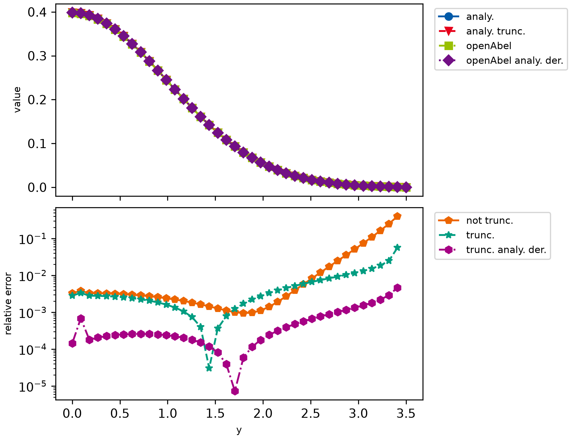
# Simple example which calculates backward Abel transform of a Gaussian.
# Results are compared with the analytical solution. Mostly default parameters are used.
############################################################################################################################################


import matplotlib.pyplot as mpl
import numpy as np
from scipy.special import erf

import openabel

############################################################################################################################################
# Plotting setup
# This block can be ignored, it's just for nicer plots.

params = {
    "axes.labelsize": 8,
    "font.size": 8,
    "legend.fontsize": 8,
    "xtick.labelsize": 10,
    "ytick.labelsize": 10,
    "text.usetex": False,
    "figure.figsize": [6.5, 5.0],
}
mpl.rcParams.update(params)
# Color scheme
colors = [
    "#005AA9",
    "#E6001A",
    "#99C000",
    "#721085",
    "#EC6500",
    "#009D81",
    "#A60084",
    "#0083CC",
    "#F5A300",
    "#C9D400",
    "#FDCA00",
]
# Plot markers
markers = ["o", "v", "s", "D", "p", "*", "h", "+", "^", "x"]
# Line styles
linestyles = ["-", "--", "-.", ":", "-", "--", "-.", ":", "-", "--", "-.", ":"]
lw = 2

############################################################################################################################################

# Parameters
n_data = 40
shift = 0.0
x_max = 3.5
sig = 1.0
step_size = x_max / (n_data - 1)
forward_backward = 1  # Backward transform, similar definition ('1' = backward) as in FFT libraries.

# Create Abel transform object, which does all precomputation possible without knowing the exact data.
abel_obj = openabel.Abel(n_data, forward_backward, shift, step_size)

# Input data
xx = np.linspace(shift * step_size, x_max, n_data)
data_in = np.exp(-0.5 * xx**2 / sig**2)

# Backward transform and analytical result.
# We show both the analytical result of a truncated Gaussian and a standard Gaussian to show
# that some error is due to truncation.
data_out = abel_obj.execute(data_in)
data_out_ana = data_in / np.sqrt(2 * np.pi) / sig
data_out_ana_trunc = data_in / np.sqrt(2 * np.pi) / sig * erf(np.sqrt((x_max**2 - xx**2) / 2) / sig)

# There is the option for the user to provide the derivative in the backward Abel transform directly.
# This is useful and can decrease the error, e.g. if the derivative can be taken analytically.
forward_backward = 2
abel_obj = openabel.Abel(n_data, forward_backward, shift, step_size)
data_in = -xx / sig**2 * np.exp(-0.5 * xx**2 / sig**2)
data_out2 = abel_obj.execute(data_in)


# Plotting
fig, axarr = mpl.subplots(2, 1, sharex=True, layout="constrained")

axarr[0].plot(xx, data_out_ana, color=colors[0], marker=markers[0], linestyle=linestyles[0], label="analy.")
axarr[0].plot(
    xx,
    data_out_ana_trunc,
    color=colors[1],
    marker=markers[1],
    linestyle=linestyles[1],
    label="analy. trunc.",
)
axarr[0].plot(xx, data_out, color=colors[2], marker=markers[2], linestyle=linestyles[2], label="openAbel")
axarr[0].plot(xx, data_out2, color=colors[3], marker=markers[3], linestyle=linestyles[3], label="openAbel analy. der.")
axarr[0].set_ylabel("value")
axarr[0].legend(loc="upper left", bbox_to_anchor=(1.02, 1.0))

axarr[1].semilogy(
    xx[:-1],
    np.abs((data_out[:-1] - data_out_ana[:-1]) / data_out_ana[:-1]),
    color=colors[4],
    marker=markers[4],
    linestyle=linestyles[4],
    label="not trunc.",
)
axarr[1].semilogy(
    xx[:-1],
    np.abs((data_out[:-1] - data_out_ana_trunc[:-1]) / data_out_ana_trunc[:-1]),
    color=colors[5],
    marker=markers[5],
    linestyle=linestyles[5],
    label="trunc.",
)
axarr[1].semilogy(
    xx[:-1],
    np.abs((data_out2[:-1] - data_out_ana_trunc[:-1]) / data_out_ana_trunc[:-1]),
    color=colors[6],
    marker=markers[6],
    linestyle=linestyles[6],
    label="trunc. analy. der.",
)
axarr[1].set_ylabel("relative error")
axarr[1].set_xlabel("y")
axarr[1].legend(loc="upper left", bbox_to_anchor=(1.02, 1.0))

mpl.savefig("example001_simple_backward.png", dpi=300)

mpl.show()