example004_full_comparison
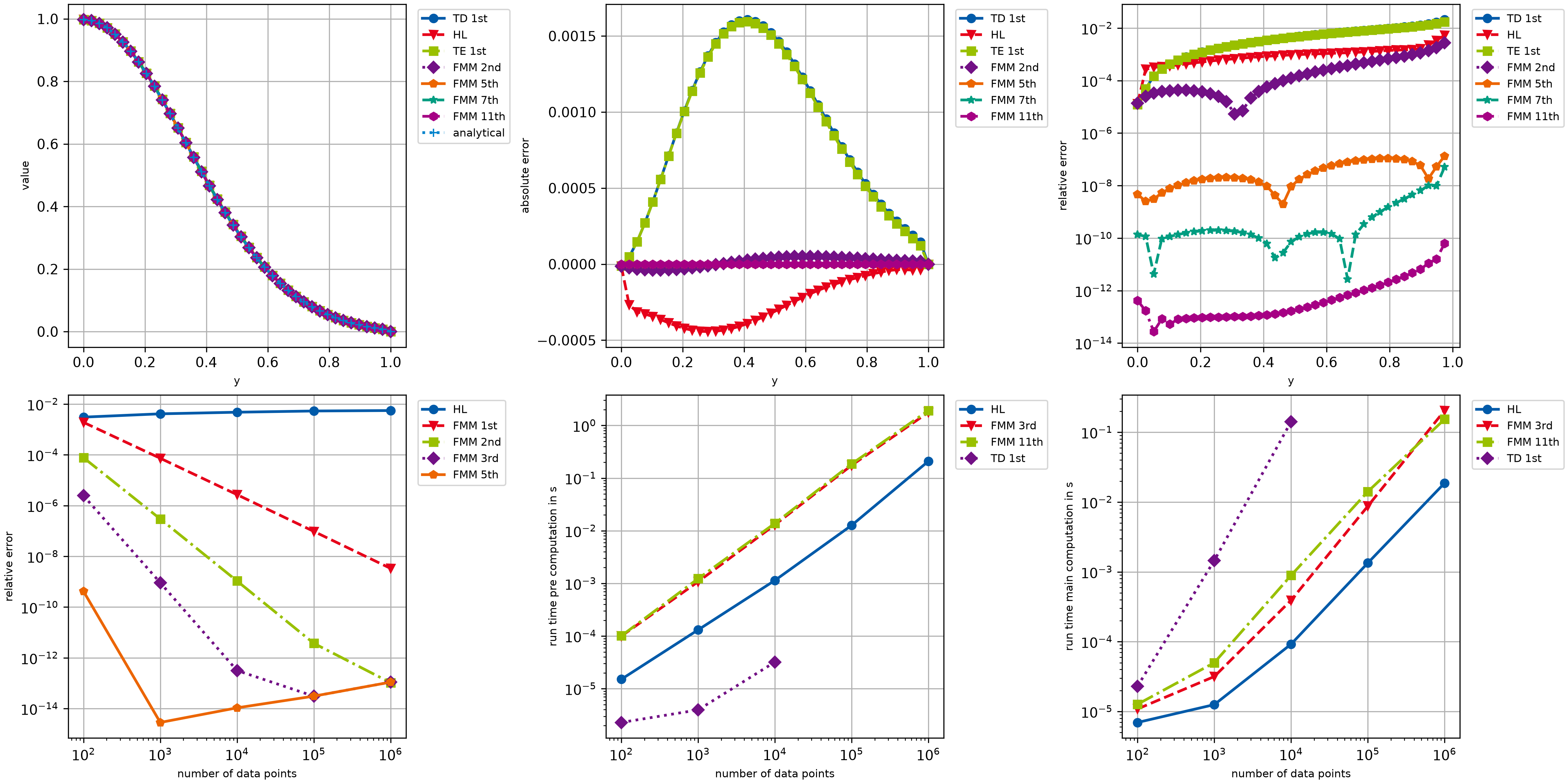
This example provides a rather extensive comparison of different openAbel methods. It shows how well the main methods perform in every regard, especially if the input data is sufficiently smooth. Most importantly one can see the fast convergence of the higher order methods in the bottom left plot, and the linear computational complexity of the main methods in the bottom middle and right plots.
############################################################################################################################################
# Example to showcase the different methods and orders, including convergence study and run times.
# Forward transform is done here, but similar results apply to the backward transform.
# This example takes possibly minutes to run, so beware
############################################################################################################################################


import time as ti

import matplotlib.pyplot as mpl
import numpy as np
from scipy.special import erf

import openabel as oa

############################################################################################################################################
# Plotting setup

params = {
    "axes.labelsize": 8,
    "font.size": 8,
    "legend.fontsize": 8,
    "xtick.labelsize": 10,
    "ytick.labelsize": 10,
    "text.usetex": False,
    "figure.figsize": [16.0, 8.0],
}
mpl.rcParams.update(params)
# Color scheme
colors = [
    "#005AA9",
    "#E6001A",
    "#99C000",
    "#721085",
    "#EC6500",
    "#009D81",
    "#A60084",
    "#0083CC",
    "#F5A300",
    "#C9D400",
    "#FDCA00",
]
# Plot markers
markers = ["o", "v", "s", "D", "p", "*", "h", "+", "^", "x"]
# Line styles
linestyles = ["-", "--", "-.", ":", "-", "--", "-.", ":", "-", "--", "-.", ":"]
lw = 2

fig, ((ax1, ax2, ax3), (ax4, ax5, ax6)) = mpl.subplots(2, 3, layout="constrained")


############################################################################################################################################
# Error over radius of different methods and orders


def error_abel(n_data, method, order):

    dx = 1.0 / (n_data - 1)
    xx = np.linspace(0.0, 1.0, n_data)
    sig = 1.0 / 3.0

    data_in = 1.0 / sig / np.sqrt(2 * np.pi) * np.exp(-0.5 * xx**2 / sig**2)

    data_ana = (
        2.0
        * 1.0
        / sig
        / np.sqrt(2 * np.pi)
        * np.exp(-0.5 * xx**2 / sig**2)
        * np.sqrt(np.pi / 2.0)
        * sig
        * erf(np.sqrt(1**2 - xx**2) / np.sqrt(2.0) / sig)
    )

    abel_obj = oa.Abel(n_data, -1, 0.0, dx, method=method, order=order)
    data_out = abel_obj.execute(data_in)

    abserr = data_out - data_ana
    relerr = np.abs(abserr / np.clip(data_ana, 1.0e-300, None))

    return (xx, abserr, relerr, data_out, data_ana)


# Loop over several methods and orders
names = ["TD 1st", "HL", "TE 1st", "FMM 2nd", "FMM 5th", "FMM 7th", "FMM 11th"]
orders = [-1, -1, 1, 2, 5, 7, 11]
methods = [0, 1, 2, 3, 3, 3, 3]

for ii in range(len(orders)):
    (xx, abserr, relerr, data_out, data_ana) = error_abel(40, methods[ii], orders[ii])
    ax1.plot(
        xx,
        data_out,
        label=str(names[ii]),
        color=colors[ii],
        linestyle=linestyles[ii],
        marker=markers[ii],
        linewidth=lw,
    )
    ax2.plot(
        xx,
        abserr,
        label=str(names[ii]),
        color=colors[ii],
        linestyle=linestyles[ii],
        marker=markers[ii],
        linewidth=lw,
    )
    ax3.semilogy(
        xx[:-1],
        relerr[:-1],
        label=str(names[ii]),
        color=colors[ii],
        linestyle=linestyles[ii],
        marker=markers[ii],
        linewidth=lw,
    )

ii += 1
ax1.plot(
    xx,
    data_ana,
    label="analytical",
    color=colors[ii],
    linestyle=linestyles[ii],
    marker=markers[ii],
    linewidth=lw,
)

ax1.legend(loc="upper left", bbox_to_anchor=(1.02, 1.0))
ax1.set_xlabel("y")
ax1.set_ylabel("value")
ax1.grid(True)

ax2.legend(loc="upper left", bbox_to_anchor=(1.02, 1.0))
ax2.set_xlabel("y")
ax2.set_ylabel("absolute error")
ax2.grid(True)

ax3.legend(loc="upper left", bbox_to_anchor=(1.02, 1.0))
ax3.set_xlabel("y")
ax3.set_ylabel("relative error")
ax3.grid(True)


############################################################################################################################################
# Convergence of different methods and orders


def convergence_abel(n_array, method, order):

    conv = np.empty(n_array.shape[0])
    for ii in range(n_array.shape[0]):
        n_data = n_array[ii]
        dx = 1.0 / (n_data - 1)
        xx = np.linspace(0.0, 1.0, n_data)
        sig = 1.0 / 3.0

        data_in = 1.0 / sig / np.sqrt(2 * np.pi) * np.exp(-0.5 * xx**2 / sig**2)

        abel_obj = oa.Abel(n_data, -1, 0.0, dx, method=method, order=order)
        data_out = abel_obj.execute(data_in)

        data_ana = (
            2.0
            / sig
            / np.sqrt(2 * np.pi)
            * np.exp(-0.5 * xx**2 / sig**2)
            * np.sqrt(np.pi / 2.0)
            * sig
            * erf(np.sqrt(1**2 - xx**2) / np.sqrt(2.0) / sig)
        )
        conv[ii] = np.sqrt(np.sum(((data_out - data_ana) / np.clip(data_ana, 1.0e-300, None)) ** 2) / n_data)

    return conv


# Loop over several methods and orders
names = ["HL", "FMM 1st", "FMM 2nd", "FMM 3rd", "FMM 5th"]
orders = [-1, 1, 2, 3, 5]
methods = [1, 3, 3, 3, 3]
n_array = 10 ** (np.arange(5) + 2)

for ii in range(len(orders)):
    conv = convergence_abel(n_array, methods[ii], orders[ii])
    ax4.loglog(
        n_array,
        conv,
        label=str(names[ii]),
        color=colors[ii],
        linestyle=linestyles[ii],
        marker=markers[ii],
        linewidth=lw,
    )

ax4.legend(loc="upper left", bbox_to_anchor=(1.02, 1.0))
ax4.set_xlabel("number of data points")
ax4.set_ylabel("relative error")
ax4.grid(True)


############################################################################################################################################
# Run times of different methods and orders


def runtimes_abel(n_array, n_measure, method, order):

    runtimes = np.zeros(n_array.shape[0])
    runtimes_pre = np.zeros(n_array.shape[0])

    for ii in range(n_array.shape[0]):
        data_in = np.ones(n_array[ii])
        timings = np.empty(n_measure)
        for jj in range(n_measure):
            t0 = ti.time()
            abel_obj = oa.Abel(n_array[ii], -1, 0.0, 1.0, method=method, order=order)
            t1 = ti.time()
            timings[jj] = t1 - t0
        runtimes_pre[ii] = np.sum(timings) / n_measure

        abel_obj = oa.Abel(n_array[ii], -1, 0.0, 1.0, method=method, order=order)
        t0 = ti.time()
        for jj in range(n_measure):
            data_out = abel_obj.execute(data_in)
        t1 = ti.time()

        runtimes[ii] = (t1 - t0) / n_measure

    return (runtimes_pre, runtimes)


# Loop over several methods and orders
names = ["HL", "FMM 3rd", "FMM 11th", "TD 1st"]
orders = [-1, 3, 11, -1]
methods = [1, 3, 3, 0]
n_array = 10 ** (np.arange(5) + 2)
n_array_small = 10 ** (np.arange(3) + 2)

for ii in range(3):
    (runtimes_pre, runtimes) = runtimes_abel(n_array, 5, methods[ii], orders[ii])
    ax5.loglog(
        n_array,
        runtimes_pre,
        label=str(names[ii]),
        color=colors[ii],
        linestyle=linestyles[ii],
        marker=markers[ii],
        linewidth=lw,
    )
    ax6.loglog(
        n_array,
        runtimes,
        label=str(names[ii]),
        color=colors[ii],
        linestyle=linestyles[ii],
        marker=markers[ii],
        linewidth=lw,
    )

for ii in range(3, len(names)):
    (runtimes_pre, runtimes) = runtimes_abel(n_array_small, 5, methods[ii], orders[ii])
    ax5.loglog(
        n_array_small,
        runtimes_pre,
        label=str(names[ii]),
        color=colors[ii],
        linestyle=linestyles[ii],
        marker=markers[ii],
        linewidth=lw,
    )
    ax6.loglog(
        n_array_small,
        runtimes,
        label=str(names[ii]),
        color=colors[ii],
        linestyle=linestyles[ii],
        marker=markers[ii],
        linewidth=lw,
    )

ax5.legend(loc="upper left", bbox_to_anchor=(1.02, 1.0))
ax5.set_xlabel("number of data points")
ax5.set_ylabel("run time pre computation in s")
ax5.grid(True)

ax6.legend(loc="upper left", bbox_to_anchor=(1.02, 1.0))
ax6.set_xlabel("number of data points")
ax6.set_ylabel("run time main computation in s")
ax6.grid(True)


mpl.savefig("example004_full_comparison.png", dpi=300)

mpl.show()